Tutorial: Reproducing the Logical Shor Noise Sweep on Neutral Atoms¶

This advanced tutorial reconstructs the simulated Shor noise sweep in Figure 9 of Rines et al., "Demonstration of a Logical Architecture Uniting Motion and In-Place Entanglement", using Clifft's five-level trajectory API and the authors' public supplementary artifact.

The reconstruction answers two questions:

Can the four published physical schedules and their logical postprocessing reproduce the paper's noise-scaling behavior in Clifft?
When is the stabilizer-compatible approximation to state-dependent transitions measurably different from exact conditional back-action?

The first question validates a realistic end-to-end leakage workflow. The second turns that reconstruction into a modeling study: it shows that an approximation can preserve decoded TVD while changing which trajectories survive postselection.

This page assumes familiarity with Clifford circuits, postselection, and the Leakage and Loss API. For a smaller first example, start with Delayed Loss in a Surface Code.

The logical experiment¶

The experiment implements a precompiled order-finding instance for N=15 and a=11. The remaining quantum workload is a three-qubit Clifford circuit with ideal output distribution

\[ P(000) = P(010) = P(101) = P(111) = \frac{1}{4}. \]

The paper realizes that logical circuit with four physical schedules:

Schedule	Physical realization	CZ gates
Unencoded	Three physical atoms	2
Two row	Two `[[4, 2, 2]]` code patches	11
Three row	Three code patches producing two samples per shot	22
Two row with LDU	Two patches plus eight leakage-detection flags	27

The [[4, 2, 2]] code detects a single physical-qubit error. Its stabilizers are XXXX and ZZZZ, so invalid codewords can be rejected but an arbitrary single error cannot be corrected. The leakage-detection unit, or LDU, adds two controlled operations and a flag measurement for each encoded data atom. A computational atom flips its flag once; a leaked atom does not participate and leaves the flag set.

Checked-in Clifft circuits¶

The four final schedules are included with the documentation:

They use Clifft's Stim-superset text format and do not require Cirq. The export preserves terminal measurement order and resolves physical atom motion into the wire labels used by later operations. A move is therefore not represented as a quantum SWAP. Its phase error appears as Z_ERROR on the atoms that arrived at their new sites.

The files record the nominal alpha=1 probabilities. The runnable script rescales the selected terms in memory, so the complete sweep needs only these four circuits. The README.md records their public source and license.

Map the five-level noise model¶

The circuits contain the Clifford operations and ordinary Pauli noise. A physical phase rotation, for example, becomes a named Clifford rotation, a twirled phase error, and an explicit level-transition site:

SQRT_Z_DAG 10
Z_ERROR(8.8823809595495095e-05) 10
LEVEL_TRANSITION[RZ_TRANSITION] 10

The effects that change or observe the atom's level live in noncomp.Model:

model = noncomp.Model(
    initial_state=INITIAL_LEVELS,
    transitions={
        "CZ": cz_transition,
        "RZ_TRANSITION": rz_transition,
    },
    classifier=noncomp.Classifier(classifier_matrix),
    reset_restores_lost=False,
    damping="exact",
)

initial_state prepares a distribution over g, e, leak_g, leak_e, and lost. Transition matrices use T[to][from]. The CZ key is a gate hook, while RZ_TRANSITION is referenced explicitly because RZ means reset in the Stim instruction set. The three-symbol classifier produces zero, one, or a heralded loss at measurement.

The full numeric matrices and classifier are kept in the runnable neutral_atom_leakage_tutorial.py. Keeping them visible there makes it possible to inspect or modify the physical model without regenerating the circuits.

Rebalanced and exact no-jump behavior¶

A transition event collapses its computational source against the live quantum state. The absence of an event also carries information when the total event rates differ between g and e. For rates \(p_g\) and \(p_e\), the surviving component receives the filter

\[ K_{\mathrm{stay}} = \sqrt{1-p_g}\lvert g\rangle\!\langle g\rvert + \sqrt{1-p_e}\lvert e\rangle\!\langle e\rvert. \]

The tutorial exposes two model choices:

matched adds a diagonal self-jump to the lower-rate computational source until the two total rates agree. The resulting no-jump filter is proportional to identity, so damping="neglect" is exact for the transformed matrices. This is the stabilizer-compatible model used for the reproduction.
exact keeps the unequal rates and uses damping="exact". Clifft applies the conditional no-jump filter and promotes coherent sites when required.

The circuit, initial population, readout model, Pauli twirls, and decoder remain the same. Only the treatment of unequal transition rates changes.

Reproduce the Figure 9 noise sweep¶

The paper varies a multiplier \(\alpha\) from 0.5 to 5. In the public model, \(\alpha\) scales the CZ phase error, physical-RZ overrotation, and movement phase error. It does not scale the transition matrices, initial level population, readout classifier, or static global-pulse error. The script keeps that distinction; alpha=1 is the nominal model stored in the circuit files.

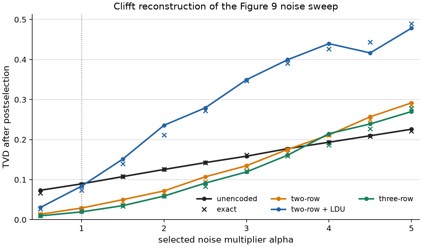
Clifft reconstruction of the Figure 9 neutral-atom Shor noise sweep

Color identifies the physical realization and lower TVD is better. Solid curves with circles use the rebalanced model; crosses use exact no-jump back-action. Each checked-in point uses 50,000 trajectories per model. The rebalanced curves reproduce the published ordering: the encoded schedules initially outperform the unencoded circuit, while their advantage disappears as the selected noise terms grow.

The exact markers mostly track the same TVD curves. The important caveat is visible at large \(\alpha\): the encoded schedules, especially the LDU circuit, accept few shots, so TVD among the survivors becomes a noisy way to compare models. Acceptance is the more sensitive observable for the approximation.

Stress-test the approximation¶

To isolate that effect, keep the real two-row LDU schedule and vary the CZ computational-rate asymmetry \(\lvert p_g-p_e\rvert\). For each point, the script preserves the mean CZ event rate and each source column's conditional distribution over jump destinations. It equalizes the smaller RZ asymmetry in both arms, leaving CZ no-jump back-action as the controlled difference.

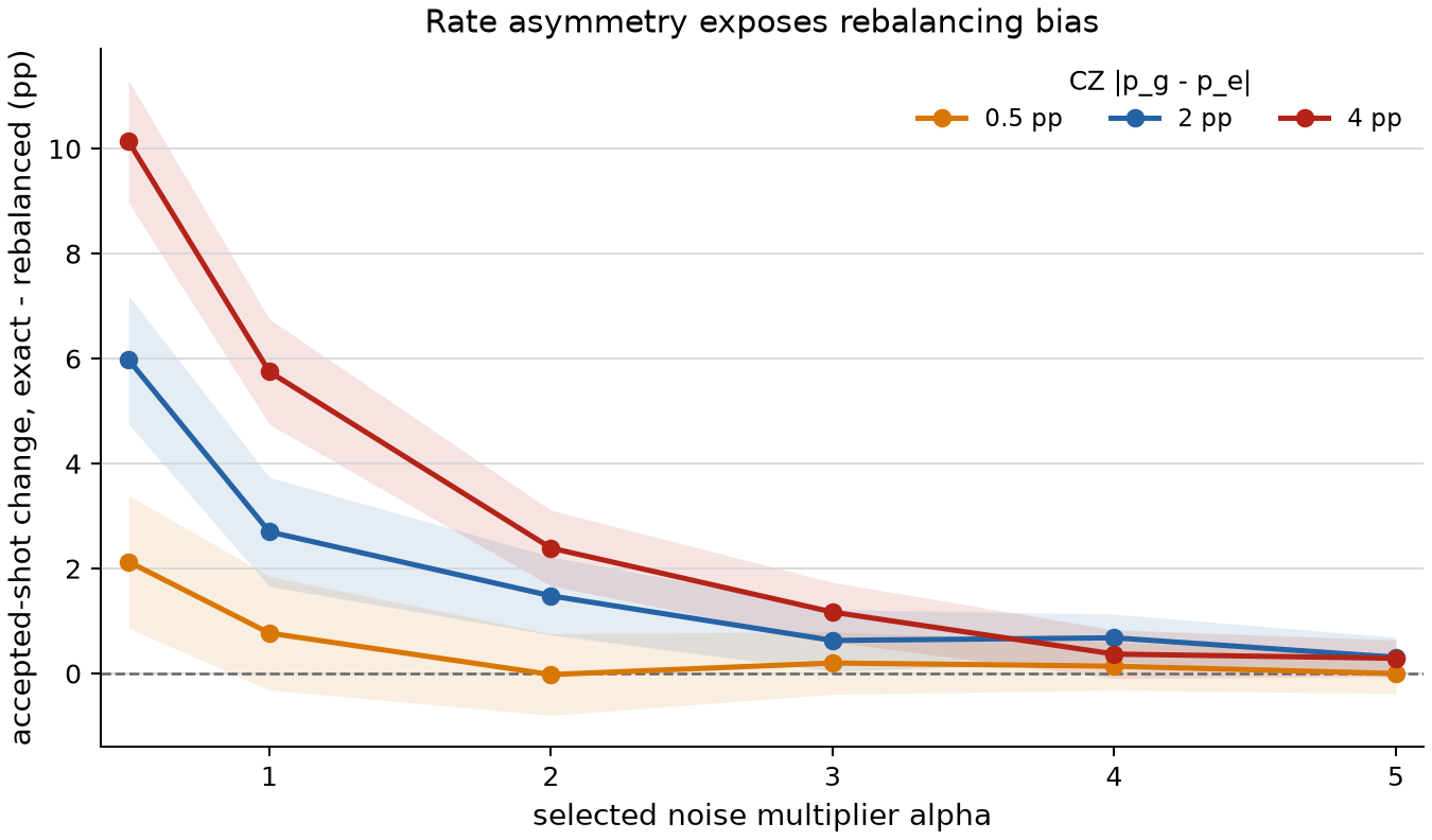
Exact-minus-rebalanced LDU acceptance under controlled CZ rate asymmetry

The vertical axis is the exact accepted-shot rate minus the rebalanced rate, in percentage points. Bands are pointwise 95% normal intervals from the two binomial acceptance estimates. The 0.5-point curve is close to the published CZ asymmetry; 2 and 4 points are hypothetical stress tests, not new hardware fits.

At low noise, the estimated shift grows with the rate asymmetry. The absolute difference eventually shrinks because very few trajectories survive either model. The checked-in figure uses 10,000 trajectories per model and point; increase --asymmetry-shots further before drawing precise quantitative conclusions. The qualitative lesson is clear: checking only decoded distributions can miss a modeling bias because conditional back-action changes the postselected ensemble itself.

The conclusion is not that the published approximation was unusable. Its physical asymmetry is mild. The useful result is that Clifft lets us validate the approximation on the actual logical workload and remove it when a device or protocol has more state-dependent transition rates.

Run the reconstruction¶

For a quick alpha=1 table across the four schedules:

uv run python docs/guide/scripts/neutral_atom_leakage_tutorial.py

To compare both no-jump models at one point:

uv run python docs/guide/scripts/neutral_atom_leakage_tutorial.py \
  --circuits two_row_ldu --models matched exact --shots 5000

To regenerate both figures at tutorial-friendly precision:

uv run --with matplotlib python \
  docs/guide/scripts/neutral_atom_leakage_tutorial.py --figures

That quick command uses 2,000 trajectories per model and Figure 9 point and 1,000 per model and asymmetry point. To reproduce the smoother checked-in figures, add --figure9-shots 50000 --asymmetry-shots 10000. Figure generation uses Clifft's automatic parallel sampling; seeded results are independent of thread count.

The script converts Clifft's measurement and herald arrays to the public artifact's three-symbol records, then:

rejects invalid preparation or LDU flags;
rejects or corrects a single loss according to the selected schedule;
decodes each valid [[4, 2, 2]] block into two logical bits; and
compares the logical Shor distribution with the ideal distribution using total variation distance.

The three-row schedule emits two logical samples per accepted physical trajectory; the reported acceptance accounts for that.

Scope and provenance¶

This is a lightweight reconstruction built from four checked-in final circuits, not a general Cirq-to-Clifft converter. It does not recreate the paper's hardware data or experimental confidence intervals. The source schedules, noise parameters, and decoder come from the Apache-2.0 supplementary artifact recorded with the circuits.

The model retains the artifact's Pauli twirls for coherent pulse errors, so the exact comparison changes the unequal-rate no-jump treatment rather than claiming a new hardware fit.

See Noncomputational States for the trajectory semantics and active-width cost of exact damping.