Tutorial: Delayed Loss in a Surface Code
This tutorial recreates the idea behind Figure 8 of Baranes et al., "Leveraging Qubit Loss Detection in Fault Tolerant Quantum Algorithms". We lose the same data qubit at two different times in a distance-3 surface-code memory experiment. Both losses are detected at the same final measurement, but they produce different detector patterns because they cancel different sets of later gates.
The example uses the paper's gate-cancellation model: after a site is lost, an operation touching it acts trivially. State-selective readout distinguishes 0, 1, and loss. These are the semantics of Clifft's lost level, operation dropping, and three-symbol measurement classifier.
This is a simulation tutorial, not a reproduction of the paper's delayed-erasure decoder or logical-error-rate results.
Prerequisites
The circuit is generated with Stim and the detector plot uses Matplotlib:
Generate the memory experiment
Start with a noiseless rotated surface-code memory-Z circuit. Flattening the REPEAT block makes it possible to place a loss at a particular round.
import matplotlib.pyplot as plt
import numpy as np
import stim

from clifft import noncomp

distance = 3
rounds = 3
data_qubit = 10

base = stim.Circuit.generated(
    "surface_code:rotated_memory_z",
    distance=distance,
    rounds=rounds,
).flattened()

print(base.get_final_qubit_coordinates()[data_qubit])
Output:
Qubit 10 is the central data site. It participates in four CX interactions per syndrome-extraction round and is not measured until the final data readout. With three extraction rounds, Stim reports four detector slices, numbered 0 through 3: an initial syndrome, two later syndrome comparisons, and the final data readout. These correspond to the four stages in the paper's example, with Stim's time coordinate starting at zero.
Select two possible loss times
The helper below inserts certain loss after that site's first CX interaction in a one-based round. The rest of the generated circuit is unchanged.
def force_loss_after_first_interaction(
    circuit: stim.Circuit,
    *,
    round_number: int,
) -> str:
    interactions_per_round = 4
    wanted_interaction = interactions_per_round * (round_number - 1) + 1
    seen_interactions = 0
    inserted = False
    lines = []

    for line in str(circuit).splitlines():
        lines.append(line)
        words = line.split()
        if words and words[0] == "CX" and str(data_qubit) in words[1:]:
            seen_interactions += 1
            if seen_interactions == wanted_interaction:
                lines.append(f"LOSS(1) {data_qubit}")
                inserted = True

    if not inserted:
        raise ValueError(f"round {round_number} is outside the generated circuit")
    return "\n".join(lines)


loss_in_round_2 = force_loss_after_first_interaction(base, round_number=2)
loss_in_round_3 = force_loss_after_first_interaction(base, round_number=3)
LOSS(1) sends the occupied site to lost with certainty. Because the destination does not depend on whether its computational source was \(\lvert 0\rangle\) or \(\lvert 1\rangle\), it also applies the correct trace-out back-action if the data qubit is entangled when it is lost.
Define state-selective readout
The classifier has one row for each possible output symbol. Computational \(\lvert 0\rangle\) and \(\lvert 1\rangle\) produce their usual binary results. The third symbol heralds a noncomputational site:
classifier = noncomp.Classifier(
    [
        [1, 0, 0, 0, 0],  # g -> 0
        [0, 1, 0, 0, 0],  # e -> 1
        [0, 0, 1, 1, 1],  # leak_g, leak_e, lost -> herald
    ]
)
model = noncomp.Model(classifier=classifier)
Only lost is reachable in this experiment. The leaked columns still need a valid classification because every classifier column is a probability distribution.
When the classifier emits the herald, Clifft marks the measurement slot in heralds and supplies a uniformly random placeholder bit to the ordinary binary record. Detectors can therefore retain their fixed shape while the out-of-band herald preserves the loss information.
Sample both histories
shots = 20_000

early = noncomp.sample(loss_in_round_2, model, shots=shots, seed=2)
late = noncomp.sample(loss_in_round_3, model, shots=shots, seed=3)

print(np.flatnonzero(early.heralds.any(axis=0)))
print(np.flatnonzero(late.heralds.any(axis=0)))
Output:
The three rounds each measure eight syndrome qubits, occupying measurement slots 0 through 23. Qubit 10 is the fifth data qubit in the final measurement, so both histories herald slot 28. From the readout alone, the two losses are indistinguishable.
Their detector records are not. The following summary counts detector locations with activation probability above 25%. Cancelled CX interactions change later stabilizer measurements, so detector comparisons that depend on them activate with probabilities near 50%. At the final time slice, two detectors also include the random placeholder for the heralded data readout.
coordinates = base.get_detector_coordinates()


def active_detector_counts(result):
    probabilities = result.detectors.mean(axis=0)
    times = sorted({int(coord[2]) for coord in coordinates.values()})
    rows = []
    for time in times:
        indices = [
            index
            for index, coord in coordinates.items()
            if int(coord[2]) == time
        ]
        active = sum(probabilities[index] > 0.25 for index in indices)
        rows.append((time, active, len(indices)))
    return rows


print("time  round-2 loss  round-3 loss")
for early_row, late_row in zip(
    active_detector_counts(early),
    active_detector_counts(late),
):
    time, early_active, total = early_row
    _, late_active, _ = late_row
    print(f"{time:>4}  {early_active:>2}/{total:<2}          {late_active:>2}/{total:<2}")
Output:
The round-2 loss changes detectors one time slice earlier. By the final readout, both histories have the same loss herald and activate the same two final-round detectors. This shared final signature is analogous to \(D_3\) in Figure 8; the paper's decoder incorporates it into the lifecycle hypergraph.
Plot the detector histories
The generated detector coordinates are (x, y, time). Plotting a spatial slice for each time step makes the difference between the two histories visible:
histories = {
    "loss in round 2": early.detectors.mean(axis=0),
    "loss in round 3": late.detectors.mean(axis=0),
}
times = sorted({int(coord[2]) for coord in coordinates.values()})

figure, axes = plt.subplots(
    len(histories),
    len(times),
    figsize=(10, 4.8),
    sharex=True,
    sharey=True,
    constrained_layout=True,
)

for row, (label, probabilities) in enumerate(histories.items()):
    for column, time in enumerate(times):
        axis = axes[row, column]
        indices = [
            index
            for index, coord in coordinates.items()
            if int(coord[2]) == time
        ]
        points = axis.scatter(
            [coordinates[index][0] for index in indices],
            [coordinates[index][1] for index in indices],
            c=[probabilities[index] for index in indices],
            cmap="magma",
            vmin=0,
            vmax=0.5,
            s=150,
            edgecolors="#303030",
            linewidths=0.7,
        )
        axis.set_title(f"t = {time}")
        axis.set_aspect("equal")
        axis.set_xlim(-0.75, 6.75)
        axis.set_ylim(6.75, -0.75)
        if column == 0:
            axis.set_ylabel(f"{label}\nspatial y")
        if row == len(histories) - 1:
            axis.set_xlabel("spatial x")

figure.colorbar(points, ax=axes, label="Detector activation probability", shrink=0.85)
figure.suptitle(f"Delayed loss of data qubit {data_qubit}", fontsize=14)
plt.show()
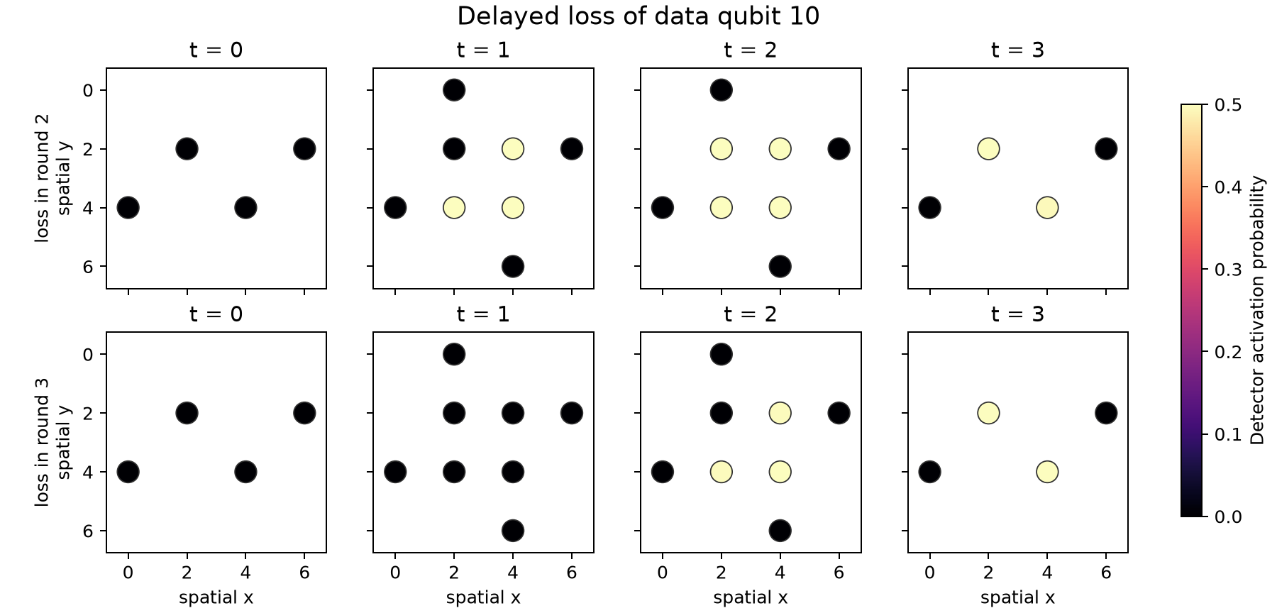
The black markers have zero activation probability. The light markers fire with probability close to one half. Both rows identify the same lost site at final readout, but their earlier spacetime patterns differ.
Let the loss time be stochastic
The known histories above isolate the effect of loss time. A physical model instead gives every entangling gate an opportunity to lose either operand.
Following the paper's independent loss model, choose the per-operand probability
so the probability that at least one of two present operands is lost is \(p_{\mathrm{gate}}\). The same transition probability applies from g and e, making its no-jump update source independent.
p_gate = 0.002
p_site = 1 - np.sqrt(1 - p_gate)

transition = [[0.0] * 5 for _ in range(5)]
transition[noncomp.Level.LOST][noncomp.Level.G] = p_site
transition[noncomp.Level.LOST][noncomp.Level.E] = p_site

stochastic_model = noncomp.Model(
    transitions={"CX": transition},
    classifier=classifier,
    reset_restores_lost=True,
)

stochastic = noncomp.sample(
    str(base),
    stochastic_model,
    shots=10_000,
    seed=7,
)

heralded = stochastic.heralds.any(axis=1)
final_loss = (stochastic.final_status == noncomp.QubitStatus.LOST).any(axis=1)

print(f"per-operand loss probability: {p_site:.7f}")
print(f"shots with detected loss: {heralded.mean():.1%}")
print(f"shots ending with a lost data site: {final_loss.mean():.1%}")
print(
    "detector activation in heralded shots: "
    f"{stochastic.detectors[heralded].mean():.1%}"
)
Output:
per-operand loss probability: 0.0010005
shots with detected loss: 13.0%
shots ending with a lost data site: 6.6%
detector activation in heralded shots: 8.1%
The CX key is a gate hook, so Clifft evaluates the transition independently for each operand after every CX. A lost syndrome qubit is classified at its round-ending MR and then restored because reset_restores_lost=True. A lost data qubit remains absent until its final measurement. This gives syndrome and data qubits the different lifecycles used by conventional syndrome extraction.
Scope of the reconstruction
This tutorial reproduces the parts of the paper's model that Clifft currently supports:
- independent loss after entangling gates;
- cancellation of later operations involving a lost site;
- delayed three-symbol state-selective readout;
- ordinary detector and observable records alongside loss heralds.
It does not implement the paper's delayed-erasure decoder. In particular, it does not construct shot-dependent superchecks or combine possible loss circuits into a decoding hypergraph. It also does not model the paper's alternative correlated loss-and-partner-error channel.
The complete runnable script is docs/guide/scripts/delayed_loss_tutorial.py:
See Leakage and Loss for the complete model API and Noncomputational States for the trajectory semantics. The advanced Logical Shor Noise Sweep tutorial shows state-dependent leakage, logical postselection, and exact no-jump back-action in a published neutral-atom experiment.