Performance
Clifft is optimized for circuits that sit between pure stabilizer simulation and fully dense statevector simulation: large circuits with mostly Clifford structure, localized non-Clifford operations, noise, measurements, detectors, and observables.
The main quantity to watch is the peak active dimension k. Non-Clifford operations can increase k, while measurements can reduce it. When k stays small relative to the total number of physical qubits, Clifft can sample large circuits exactly at high throughput.
Summary
| Regime | Recommended tool | What the benchmarks show |
|---|---|---|
| Pure Clifford QEC | Stim | Stim remains faster for fully Clifford circuits. Clifft is useful here mainly when you want one workflow that also supports nearby non-Clifford variants. |
| Low-magic / near-Clifford FT circuits | Clifft | Clifft gives its largest gains when non-Clifford effects remain localized and frequent measurements keep k small. |
| Dense universal circuits | Statevector tools or Clifft | When k = n, Clifft behaves like a dense statevector simulator and remains competitive with leading CPU simulators. |
Clifft is not intended to replace Stim for fully Clifford workloads. Its main target is the middle regime where exact non-Clifford effects matter, but the non-Clifford activity remains small enough to avoid full dense-statevector scaling.
QEC benchmark throughput
The table below reports sample-time throughput in effective shots per second. kmax is the peak active virtual dimension reached during execution. For near-Clifford circuits, this is often a better predictor of Clifft performance than the total qubit count or raw non-Clifford operation count.
| Circuit | Qubits | Ops | Non-Clifford ops | kmax | Clifft | Stim | Tsim |
|---|---|---|---|---|---|---|---|
Surface code d=7, r=7 | 118 | 4,667 | 0 | 0 | 2.2M | 20.1M | 314.7k |
Cultivation d=3 | 15 | 676 | 29 | 4 | 10.4M | — | 27.9k |
Cultivation d=5 | 42 | 4,379 | 91 | 10 | 314.4k | — | DNC |
| Distillation | 85 | 1,163 | 10 | 5 | 1.5M | — | 1.5M |
Surface code d=3, r=1 with coherent noise | 26 | 173 | 65 | 5 | 19.4M | — | 14.4M |
Surface code d=3, r=3 with coherent noise | 26 | 415 | 195 | 8 | 1.7M | — | DNC |
Surface code d=5, r=1 with coherent noise | 64 | 533 | 209 | 13 | 133.1k | — | 570.9k |
Surface code d=5, r=5 with coherent noise | 64 | 2,073 | 1,045 | 24 | 0.7 | — | DNC |
DNC means the circuit did not compile within the benchmark time limit. Stim entries are shown as — for non-Clifford circuits because Stim does not support those operations directly.
These numbers should be read as representative benchmark points, not as universal performance guarantees. Throughput depends on the circuit structure, noise model, measurement schedule, active dimension, and hardware.
Interpreting the results
Pure Clifford circuits
For fully Clifford circuits, Stim remains the right tool. It is purpose-built for that regime and can vectorize stabilizer-frame work across many shots.
Clifft pays some overhead to maintain the frame-factored representation even when kmax = 0. The benefit is that the same workflow can also support non-Clifford variants of the circuit.
Low-magic fault-tolerant circuits
This is Clifft's main target regime. In circuits such as magic-state cultivation, the physical circuit can involve many operations and many qubits, but the non-Clifford effects remain localized. Frequent measurements can also shrink the active state during execution.
In this setting, Clifft can avoid dense-statevector scaling in the full physical qubit count and instead operate on the smaller active state.
Coherent-noise and larger-k circuits
The coherent-noise benchmarks show how performance changes as kmax grows. As the active dimension increases, Clifft gradually transitions toward dense statevector behavior. This is expected: active-state operations scale exponentially in k.
The important point is that the transition is controlled by the active dimension, not simply by the total number of physical qubits.
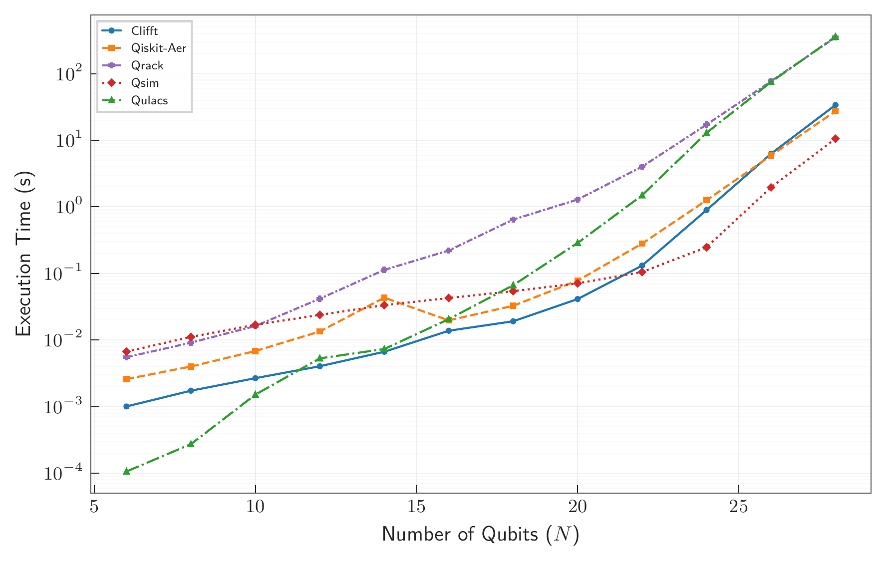
Dense-statevector limit
When k = n, Clifft no longer benefits from near-Clifford structure and behaves like a dense statevector simulator. This is not its primary target regime, but it is still useful to understand the worst case.
On random Quantum Volume circuits at depth D = N, Clifft remains competitive with leading CPU statevector simulators such as Qiskit Aer, qsim, Qrack, and Qulacs.
Hardware and methodology notes
The benchmark table reports sample-time throughput. Clifft and Stim were run on a single cloud CPU instance, while Tsim was run on a GPU instance. The benchmark values are intended to compare practical throughput on representative hardware, not to isolate every architectural difference between CPUs and GPUs.
Compilation time is amortized for Clifft and Stim. For the QEC circuits shown above, Clifft compilation is small compared with repeated sampling. Tsim numbers exclude compilation time and a warmup run.
Some simulators are sensitive to physical noise rate, circuit structure, and backend-specific optimizations. In particular, non-Clifford operation count alone is not enough to predict performance. For Clifft, the most important quantities are the active dimension k, how long the circuit spends at each active dimension, and whether measurements collapse the active state.
Reproducing benchmarks
The full benchmark methodology, hardware details, circuits, and analysis scripts are described in the Clifft paper and companion benchmark repository.
- Paper: https://arxiv.org/abs/2604.27058
- Benchmark circuits and scripts: clifft-paper