Tutorial: Importance Sampling Magic State Cultivation
Estimating logical error rates of quantum error-correcting codes at low physical error rates requires sampling rare events. With standard Monte Carlo, the number of shots needed to resolve a logical error rate \(p_L\) scales as \(O(1 / p_L)\), so direct simulation becomes increasingly expensive as \(p_L\) decreases.
Stratified importance sampling solves this by conditioning on the number of physical faults \(k\) that occur in a single shot. By running dedicated shot batches at each fault count \(k\) and weighting the results by the exact probability \(P(K = k)\), we can estimate \(p_L\) with dramatically fewer total shots.
This tutorial walks through Clifft's importance sampling API for the distance-3 magic state cultivation protocol from Craig Gidney, Noah Shutty, and Cody Jones, "Magic state cultivation: growing T states as cheap as CNOT gates" (arXiv:2409.17595). It focuses on simulating the injection and escape stages of the protocol. We recreate the importance sampling analysis for this problem from Thomas Tuloup and Thomas Ayral, "Computing logical error thresholds with the Pauli Frame Sparse Representation" (arXiv:2603.14670), and use the d=3 T-gate and S-gate circuits distributed with Riling Li et al., "SOFT: A High-Performance Simulator for Universal Fault-Tolerant Quantum Circuits" (arXiv:2512.23037).
This is an advanced tutorial. It assumes familiarity with detector-based QEC circuits, post-selection, and logical error-rate estimation.
Overview
The workflow has four steps:
- Compile a noisy circuit and extract per-site fault probabilities
- Compute the Binomial PMF \(P(K = k)\)
- Sample each stratum with
sample_k_survivors - Combine results with the stratified estimator
A bonus step shows how to reweight the same simulation data to sweep over physical error rates without re-simulating.
The Circuit
We use two d=3 magic state cultivation circuits, each operating on 15 qubits:
- T-gate circuit (
circuit_d3_t_gate_p0.001.stim): Contains T/T_DAG gates (non-Clifford), which standard Clifford simulators like Stim cannot handle. Clifft compiles and simulates the actual T-state preparation circuit natively. - S-gate circuit (
circuit_d3_s_gate_p0.001.stim): Contains S/S_DAG gates (Clifford). Tuloup and Ayral used this proxy circuit because Stim is Clifford-only. It provides a useful comparison point with the full T-gate protocol.
Both circuits share the same structure: 15 qubits, 20 detectors, 1 observable, and 518 noise sites at uniform \(p = 0.001\).
Step 1: Compile and Inspect
import numpy as np
import clifft

# Load the circuit
with open("docs/guide/circuits/circuit_d3_t_gate_p0.001.stim") as f:
    circuit_text = f.read()

# Build an all-detector postselection mask.
# Magic state cultivation discards any shot where a detector fires.
prog_probe = clifft.compile(
    circuit_text,
    normalize_syndromes=True,
    hir_passes=clifft.default_hir_pass_manager(),
    bytecode_passes=clifft.default_bytecode_pass_manager(),
)
num_det = prog_probe.num_detectors

mask = [1] * num_det  # one flag per detector

# Compile with postselection
prog = clifft.compile(
    circuit_text,
    normalize_syndromes=True,
    postselection_mask=mask,
    hir_passes=clifft.default_hir_pass_manager(),
    bytecode_passes=clifft.default_bytecode_pass_manager(),
)

print(f"Peak rank:      {prog.peak_rank}")       # 4 (only 2^4 = 16 amplitudes)
print(f"Detectors:      {prog.num_detectors}")    # 20
print(f"Observables:    {prog.num_observables}")   # 1

# Extract per-site fault probabilities
site_probs = prog.noise_site_probabilities
print(f"Noise sites:    {len(site_probs)}")       # 518
print(f"All uniform:    {len(np.unique(site_probs)) == 1}")  # True
print(f"Site prob:      {site_probs[0]}")         # 0.001
The noise_site_probabilities property returns a 1D array covering all fault sites: quantum noise sites (multi-channel Pauli errors) followed by readout noise entries (bit-flip errors). For the cultivation circuit, all 518 sites share the same probability \(p = 0.001\).
Step 2: Compute the PMF
The total fault count \(K\) follows the Binomial distribution for these circuits because all fault sites share the same physical error rate:
Clifft exposes the per-site probabilities through program.noise_site_probabilities. We can verify they are uniform, then compute the PMF directly:
from scipy.stats import binom

max_k = 16
assert np.allclose(site_probs, site_probs[0])
P_K = binom.pmf(np.arange(max_k + 1), len(site_probs), site_probs[0])

for k in range(max_k + 1):
    print(f"  P(K={k:2d}) = {P_K[k]:.4e}")
print(f"  Tail P(K>{max_k}) = {1.0 - sum(P_K):.2e}")
Output:
  P(K= 0) = 5.9556e-01
  P(K= 1) = 3.0881e-01
  P(K= 2) = 7.9907e-02
  P(K= 3) = 1.3758e-02
  P(K= 4) = 1.7731e-03
  P(K= 5) = 1.8245e-04
  P(K= 6) = 1.5615e-05
  P(K= 7) = 1.1433e-06
  P(K= 8) = 7.3102e-08
  P(K= 9) = 4.1466e-09
  P(K=10) = 2.1127e-10
  P(K=11) = 9.7667e-12
  P(K=12) = 4.1306e-13
  P(K=13) = 1.6093e-14
  P(K=14) = 5.8110e-16
  P(K=15) = 1.9544e-17
  P(K=16) = 6.1504e-19
  Tail P(K>16) = 7.77e-16
At \(p = 0.001\) with 518 sites, the expected fault count is \(\mu = Np \approx 0.518\), so most shots have 0 or 1 faults. Strata beyond \(k \approx 6\) have negligible weight at this \(p\), but we sample up to \(k = 16\) to support reweighting at higher physical error rates (e.g., \(p = 0.01\) where \(\mu \approx 5.2\)).
Step 3: Stratified Sampling
Use sample_k_survivors to run shots with exactly \(k\) forced faults. The function draws the \(k\) fault locations from the exact conditional Poisson-Binomial distribution. When all site probabilities are equal (as detected automatically), it uses an efficient \(O(k)\) Fisher-Yates sampler.
shots_per_k = 750_000
stratum_data = []

for k in range(max_k + 1):
    result = clifft.sample_k_survivors(prog, shots=shots_per_k, k=k, seed=42 + k)
    stratum_data.append({
        "k": k,
        "total": result.total_shots,
        "passed": result.passed_shots,
        "errors": result.logical_errors,
    })
This should run quickly on most machines, simulating 12.75 million shots across 17 strata.
Combining with the Stratified Estimator
For circuits with postselection, the survival probability depends on \(k\), so numerator and denominator must be weighted separately:
where \(\hat{p}_{\text{fail}|k} = \text{errors}_k / \text{shots}_k\) and \(\hat{p}_{\text{surv}|k} = \text{passed}_k / \text{shots}_k\):
weighted_errors = 0.0
weighted_survival = 0.0

for d in stratum_data:
    k = d["k"]
    total = d["total"]
    if total == 0 or P_K[k] < 1e-30:
        continue
    weighted_errors += P_K[k] * d["errors"] / total
    weighted_survival += P_K[k] * d["passed"] / total

p_fail = weighted_errors / weighted_survival
print(f"Importance sampling estimate: p_fail = {p_fail:.4e}")
Output:
The logical error rate is roughly \(10^{-6}\). Clifft is fast enough that brute-force Monte Carlo is still possible here, but it would need far more shots to reach comparable precision. This is where importance sampling helps: we captured enough error events across strata to produce a meaningful estimate with only 12.75M total shots.
Per-Stratum Analysis
The real power of importance sampling is the per-stratum decomposition. The plot below shows the Binomial PMF at two physical error rates (left axis, bars) alongside the conditional error rate \(p_{\text{fail}|k}\) (right axis, red line):
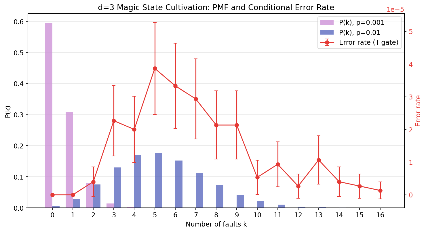
Key observations:
- k=0 and k=1 have zero logical errors: with fewer than 2 faults, the cultivation protocol's postselection catches all bad shots.
- The error rate peaks around k=5--6 at roughly \(4 \times 10^{-5}\), then gradually declines at higher k as postselection becomes more aggressive (fewer survivors means fewer opportunities for errors).
- The PMF shifts right when \(p\) increases from 0.001 to 0.01, but the red error rate curve stays fixed -- it depends only on the circuit structure, not on \(p\).
The weighted contributions \(P(K=k) \cdot p_{\text{fail}|k}\) show where the logical error rate actually comes from:
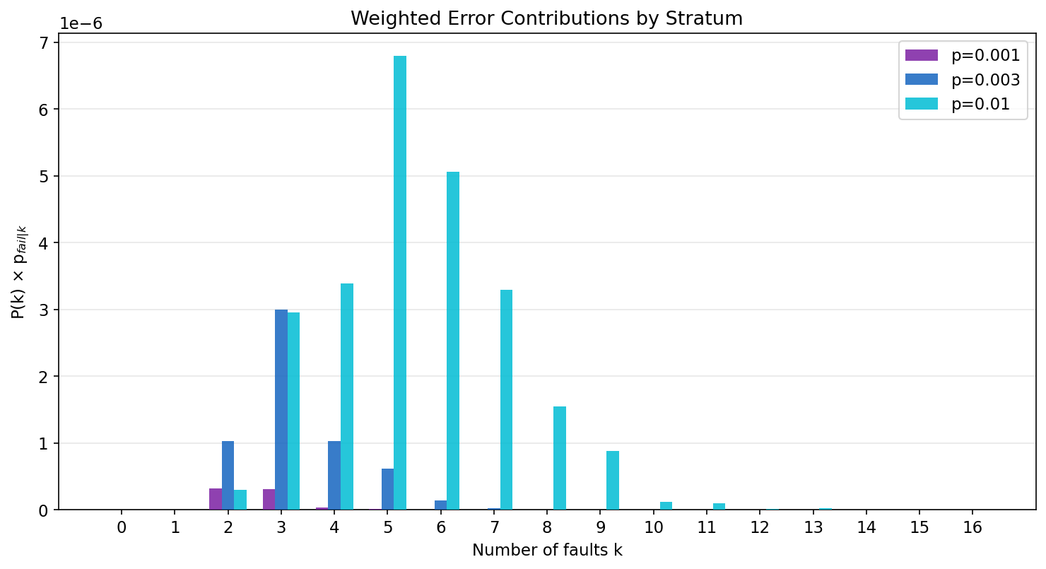
At \(p = 0.001\) (purple), the dominant contribution comes from k=2--3. As \(p\) increases to 0.01 (cyan), the "danger zone" shifts to k=5--6 where both the PMF weight and the error rate are substantial.
Step 4: Error Rate Sweep via Reweighting
A key insight from Tuloup & Ayral (2026): since the conditional error rate \(p_{\text{fail}|k}\) depends on the circuit structure (which fault locations exist and what they do) but not on the physical error rate \(p\), we can reweight the same simulation results with different PMFs to sweep over \(p\) without re-simulating.
For a circuit where all \(N\) noise sites share the same probability \(p\), the PMF reduces to the Binomial distribution \(P(K=k) = \binom{N}{k} p^k (1-p)^{N-k}\). We also compute error bars using the variance of the stratified estimator numerator (Eq. 55 from Tuloup & Ayral):
Since the survival rate has negligible statistical uncertainty compared to the rare error rate, we divide the standard error of the numerator by the survival rate to get the final confidence interval.
from scipy.stats import binom

p_values = [0.001, 0.002, 0.003, 0.005, 0.007, 0.01]
N = len(site_probs)

for p in p_values:
    pmf = binom.pmf(np.arange(max_k + 1), N, p)
    w_err = sum(pmf[d["k"]] * d["errors"] / d["total"]
                for d in stratum_data if d["total"] > 0)
    w_surv = sum(pmf[d["k"]] * d["passed"] / d["total"]
                 for d in stratum_data if d["total"] > 0)
    # Variance of the numerator (Eq. 55)
    var_num = sum(pmf[d["k"]]**2 * (d["errors"]/d["total"])
                  * (1.0 - d["errors"]/d["total"]) / d["total"]
                  for d in stratum_data if d["total"] > 0)
    rate = w_err / w_surv if w_surv > 0 else 0.0
    ci = 1.96 * (var_num**0.5 / w_surv) if w_surv > 0 else 0.0
    disc = 1.0 - w_surv / sum(pmf)
    print(f"  p={p:.4f}: p_fail={rate:.3e} +/- {ci:.3e}, discard={disc*100:.1f}%")
Output:
  p=0.0010: p_fail=9.822e-07 +/- 5.698e-07, discard=31.3%
  p=0.0020: p_fail=5.821e-06 +/- 2.394e-06, discard=52.8%
  p=0.0030: p_fail=1.792e-05 +/- 5.912e-06, discard=67.5%
  p=0.0050: p_fail=8.439e-05 +/- 2.051e-05, discard=84.5%
  p=0.0070: p_fail=2.620e-04 +/- 5.229e-05, discard=92.6%
  p=0.0100: p_fail=9.812e-04 +/- 1.690e-04, discard=97.5%
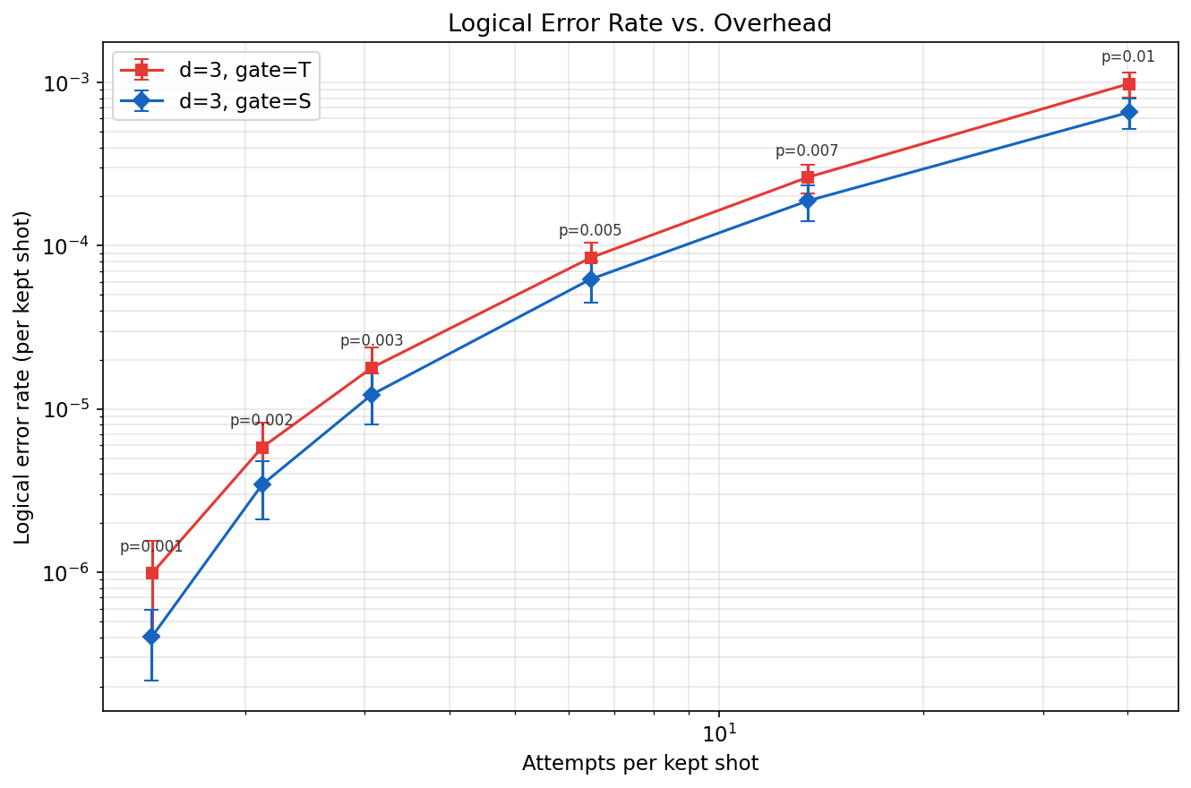
The plot above shows both the T-gate (red squares) and S-gate (blue diamonds) cultivation circuits. A single simulation run per circuit (12.75M shots each, ~18 seconds for T and faster for S) produced the complete error rate curves with 95% confidence intervals across 6 physical error rates.
The x-axis shows "attempts per kept shot" -- the overhead cost of postselection. Key observations:
- The S-gate circuit achieves a much lower logical error rate than the T-gate circuit at every physical error rate, consistent with the fact that S gates are Clifford operations and easier to cultivate.
- At \(p = 0.01\), it takes ~40 attempts to produce one surviving shot for both circuits, but the T-gate error rate (~\(10^{-3}\)) is orders of magnitude higher than the S-gate rate.
- Both curves were generated from the same reweighting approach -- no re-simulation needed to sweep across \(p\) values.
API Reference
clifft.sample_k(program, shots, k, seed=None)
Sample with exactly k forced faults per shot. Returns a SampleResult, just like clifft.sample(). Results must be weighted by \(P(K=k)\) for correct error rate estimation.
For programs with post-selection, use clifft.sample_k_survivors(...) instead. Fixed-row output from sample_k(...) cannot represent discarded shots.
Raises ValueError if the stratum has zero probability mass (e.g., k exceeds the number of non-zero-probability sites).
clifft.sample_k_survivors(program, shots, k, seed=None, keep_records=False)
Sample survivors with exactly k forced faults per shot. Returns a SampleResult whose .measurements, .detectors, and .observables arrays contain only surviving shots. Survivor metadata is available via .total_shots, .passed_shots, .discards, .logical_errors, and .observable_ones.
Raises ValueError if the stratum has zero probability mass.
program.noise_site_probabilities
1D numpy array of per-site total fault probabilities. Quantum noise sites (sum of channel probabilities) come first, followed by readout noise entries. Use for computing the fault-count PMF.
Generating the Plots
The plots in this tutorial can be reproduced with the script at docs/guide/scripts/importance_sampling_tutorial.py:
Further Reading
- Gidney, Shutty, and Jones (2024), "Magic state cultivation: growing T states as cheap as CNOT gates" (arXiv:2409.17595).
- Tuloup & Ayral (2026), "Computing logical error thresholds with the Pauli Frame Sparse Representation" (arXiv:2603.14670) -- introduced subset importance sampling for magic state cultivation.
- Li et al. (2025), "SOFT: A High-Performance Simulator for Universal Fault-Tolerant Quantum Circuits" (arXiv:2512.23037) -- source of the cultivation circuits used here.