Benchmark: Clifft vs Qiskit-Aer¶

Clifft's factored-state architecture means simulation cost scales with the circuit's non-Clifford complexity (the active dimension \(k\), also called the active rank), not the total qubit count \(N\). This page compares Clifft against Qiskit-Aer's state vector simulator on two parameter sweeps that isolate each scaling axis. This is a small, locally reproducible benchmark designed to isolate Clifft's scaling behavior.

Circuit Design¶

The benchmark circuit has three parameters:

• N — total physical qubits
• k — active dimension (number of qubits that receive non-Clifford T-gates)
• t — total T-gates applied

The circuit places T-gates interleaved with Hadamard and CNOT gates on the first \(k\) qubits, then pads the remaining \(N - k\) qubits with a Clifford entangling layer (Hadamards followed by a CNOT chain across all \(N\) qubits).

A dense state vector simulator like Qiskit-Aer must allocate \(2^N\) complex amplitudes regardless of circuit structure. Clifft's compiler recognizes that the Clifford padding can be absorbed into an offline Clifford frame \(U_C\), so its virtual machine only allocates \(2^k\) amplitudes.

Two Sweeps¶

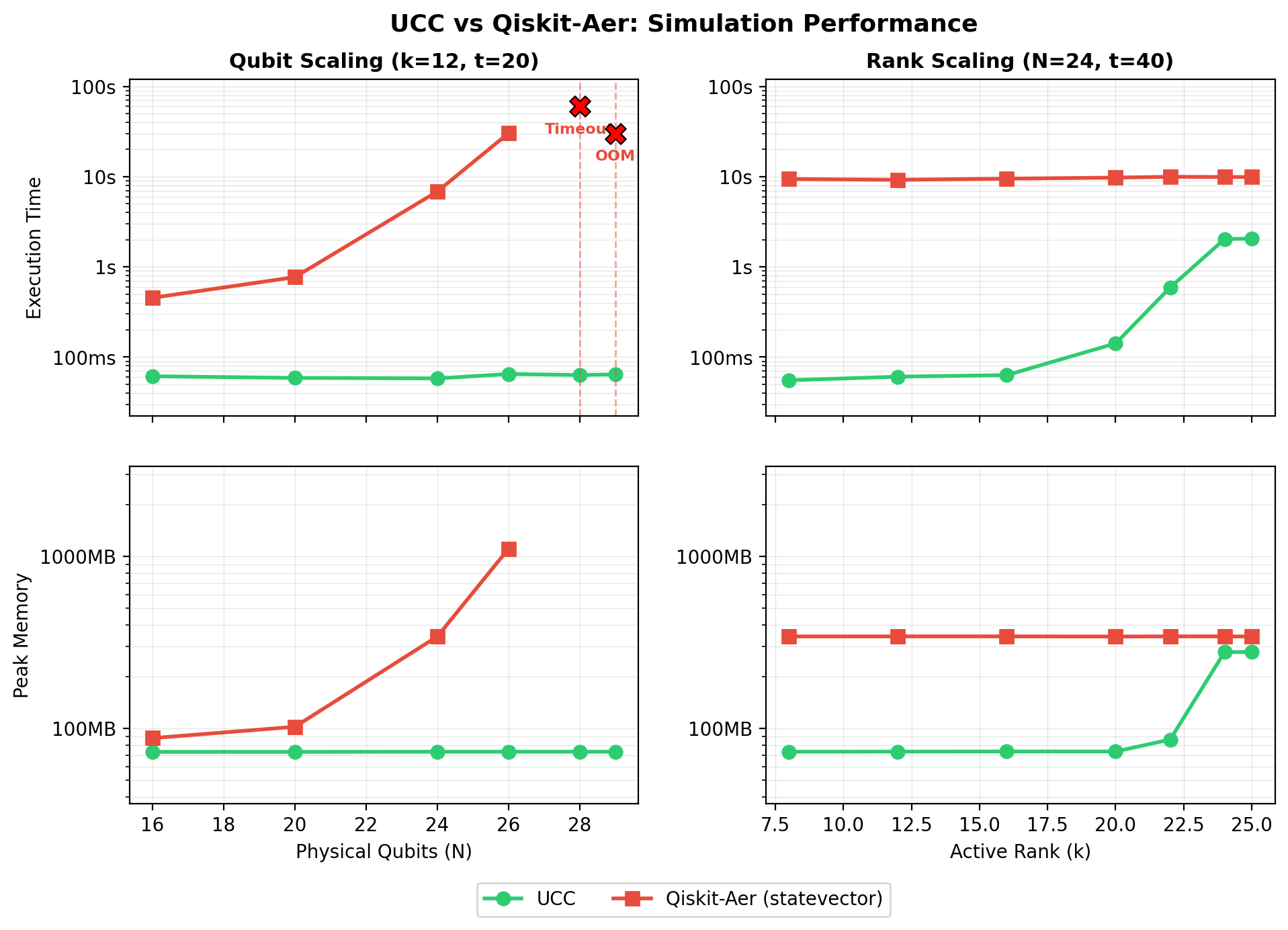
Qubit Scaling (left panels)¶

Fix \(k = 12\) and \(t = 20\), sweep \(N\) from 16 to 29.

• Clifft stays flat at ~60ms and ~73MB regardless of \(N\), because its active array is always \(2^{12}\).
• Qiskit-Aer doubles in time and memory with each additional qubit. It times out at \(N = 28\) (>120s) and exceeds available RAM at \(N = 29\).

Active-Dimension Scaling (right panels)¶

Fix \(N = 24\) and \(t = 40\), sweep \(k\) from 8 to 25.

• Qiskit-Aer is constant at ~10s and ~343MB, since it always tracks \(2^{24}\) amplitudes.
• Clifft scales as \(O(2^k)\). For small \(k\) it is over 100x faster; by \(k = 24\) the two converge because Clifft's active array approaches Qiskit's full state vector.

This is the honest tradeoff: Clifft wins when \(k \ll N\), which is the regime relevant to most error-corrected and near-term circuits where Clifford gates dominate.

Prerequisites¶

pip install clifft qiskit qiskit-aer matplotlib

Running the Benchmark¶

The benchmark script is self-contained. It generates circuits in Qiskit, converts them to Stim format for Clifft, runs both simulators in isolated subprocesses (for clean memory measurement), and produces the plot.

# Run full benchmark and generate plot
python docs/guide/scripts/run_benchmark.py

# Re-plot from existing results without re-running
python docs/guide/scripts/run_benchmark.py --plot-only

# Custom output path
python docs/guide/scripts/run_benchmark.py -o my_plot.png

On an 8GB machine, the full sweep takes approximately 5-10 minutes. Qiskit will naturally time out or OOM on the larger qubit counts.

Why Clifft Is Faster at Low Active Dimension¶

The key insight is Clifft's factored-state representation:

The compiler absorbs all Clifford gates into the offline Clifford frame \(U_C\). Only the active subspace \(|\phi\rangle_A\) (dimension \(2^k\)) is stored and evolved by the virtual machine. At runtime the VM maintains only the active state vector and a lightweight Pauli frame \(P\) (updated by XOR for conditional Paulis and noise); \(U_C\) is not tracked online. The dormant qubits \(|0\rangle_D\) cost nothing at runtime.

Qiskit-Aer has no such factorization — it must allocate and evolve a full \(2^N\) state vector for every circuit.